Image Segmentation and Obstacle Detection from RGB Video Using a Neural Network
Overview
In this project, I worked with two other MSR students to build an neural network using Pytorch to detect obstacles in the path of a mobile robot. I then deployed the trained network on the Autonomous RC Car I built to test it. Currently, I am working on using the trained network to further improve the lane centering abilities of the autonomous car while navigating through hallways, classrooms, and labs.
Video Demo
Below is sample video captured while testing the network on the autonomous car robot. In this video, “safe” areas are marked in black, obstacles and unsafe areas are marked in white. In this video, it is clear that the robot is able to distinguish between walls and floors. It also seems to be able to detect some obstacles, like shoes of someone walking in front of it, but it struggles with other obstacles that were not in the training dataset. This will likely be improved with a more robust and diverse training dataset. More training time could improve these issues as well.
Neural Network Architecture
The architecture of this neural network is based on the deep convolutional neural network SegNet, proposed by Vijay Badrinarayanan, Alex Kendall, Roberto Cipolla with some changes to better suit this application. This network is designed to map RGB images to segmented masks.
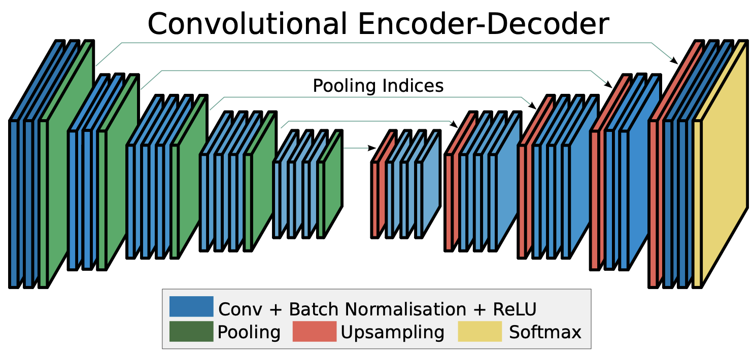
In our model, each encoder block includes the following layers:
- Convolution layer 1 (Conv2d)
- Convolution layer 2 (Conv2d)
- Batch Normalization layer (BatchNorm2d)
- Non-Linear Activation layer (ReLU)
- Pooling layer (MaxPool)
And each decoder block includes:
- Upsampling layer (UpsamplingNearest2d)
- Convolution layer 1 (Conv2d)
- Convolution layer 2 (Conv2d)
- Batch Normalization layer (BatchNorm2d)
- Non-Linear Activation layer (ReLU)
Compared to the architecture proposed in the paper, this model uses one less block for encoding and decoding. Additionally, we use only two convolutional layer in each block, while the paper uses three. We are only doing binary image segmentation, while the paper segments images into several regions. For this application, the extra complexity is not needed, and the simpler model trained more quickly and was easier to iterate on.
Below is the full model architecture, as output by the torchsummary Python library for a 240x240 image.
----------------------------------------------------------------
        Layer (type)               Output Shape         Param #
================================================================
            Conv2d-1         [16, 32, 240, 240]           2,432
            Conv2d-2         [16, 32, 240, 240]          25,632
    BatchNorm2d-3         [16, 32, 240, 240]              64
            ReLU-4         [16, 32, 240, 240]               0
        MaxPool2d-5         [16, 32, 120, 120]               0
            Conv2d-6         [16, 32, 120, 120]          25,632
            Conv2d-7         [16, 32, 120, 120]          25,632
    BatchNorm2d-8         [16, 32, 120, 120]              64
            ReLU-9         [16, 32, 120, 120]               0
        MaxPool2d-10           [16, 32, 60, 60]               0
        Conv2d-11           [16, 64, 60, 60]          51,264
        Conv2d-12           [16, 64, 60, 60]         102,464
    BatchNorm2d-13           [16, 64, 60, 60]             128
            ReLU-14           [16, 64, 60, 60]               0
        MaxPool2d-15           [16, 64, 30, 30]               0
        Conv2d-16          [16, 128, 30, 30]         204,928
        Conv2d-17          [16, 128, 30, 30]         409,728
    BatchNorm2d-18          [16, 128, 30, 30]             256
            ReLU-19          [16, 128, 30, 30]               0
        MaxPool2d-20          [16, 128, 15, 15]               0
UpsamplingNearest2d-21          [16, 128, 30, 30]               0
        Conv2d-22           [16, 64, 30, 30]         204,864
        Conv2d-23           [16, 64, 30, 30]         102,464
    BatchNorm2d-24           [16, 64, 30, 30]             128
            ReLU-25           [16, 64, 30, 30]               0
UpsamplingNearest2d-26          [16, 128, 60, 60]               0
        Conv2d-27           [16, 32, 60, 60]         102,432
        Conv2d-28           [16, 32, 60, 60]          25,632
    BatchNorm2d-29           [16, 32, 60, 60]              64
            ReLU-30           [16, 32, 60, 60]               0
UpsamplingNearest2d-31         [16, 64, 120, 120]               0
        Conv2d-32         [16, 32, 120, 120]          51,232
        Conv2d-33         [16, 32, 120, 120]          25,632
    BatchNorm2d-34         [16, 32, 120, 120]              64
            ReLU-35         [16, 32, 120, 120]               0
UpsamplingNearest2d-36         [16, 64, 240, 240]               0
        Conv2d-37          [16, 3, 240, 240]           4,803
        Conv2d-38          [16, 2, 240, 240]             152
    BatchNorm2d-39          [16, 2, 240, 240]               4
            ReLU-40          [16, 2, 240, 240]               0
================================================================
Total params: 1,365,695
Trainable params: 1,365,695
Non-trainable params: 0
----------------------------------------------------------------
Input size (MB): 10.55
Forward/backward pass size (MB): 2380.08
Params size (MB): 5.21
Estimated Total Size (MB): 2395.83
----------------------------------------------------------------
Dataset Creation
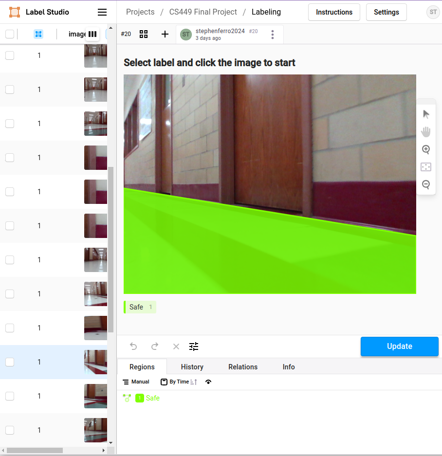
To create the dataset, we drove the robot through hallways and labs using tele-op control while collecting and saving images from the camera. We then used the labeling tool LabelStudio to mark the “safe” regions for the robot to travel to in a selection of images.
Once the initial dataset was created, we also augmented the dataset by duplicating and modifying the original images. For each original image, we did the following:
- Crop each photo three times (shift left, centered, shift right)
- Created a mirrored copy of all images
- Copy each image and randomly adjust the HSV values
- Copy each images and add random white noise
Using these methods, we increased our initial dataset of ~300 labelled images to >7000. This made our training data much more robust and led to more reliable results.
Below are examples of a training image:
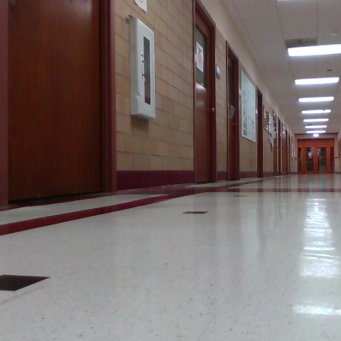
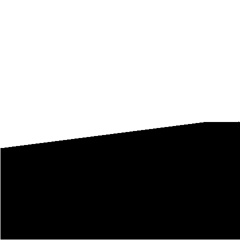
And here it’s is binary image label, where black regions are “safe” and white indicates “unsafe”:
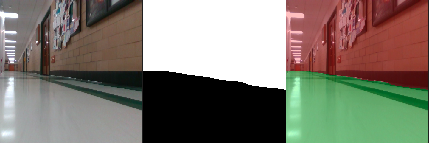
Initial Results
Below, you can see initial results from the deploying the trained dataset on the robot. When compared to the label image, the output mask had 97% accuracy - that is, 97% of the pixels matched the label. in scenarios like this, where the model is primarily identifying walls, it tends to work very reliably.
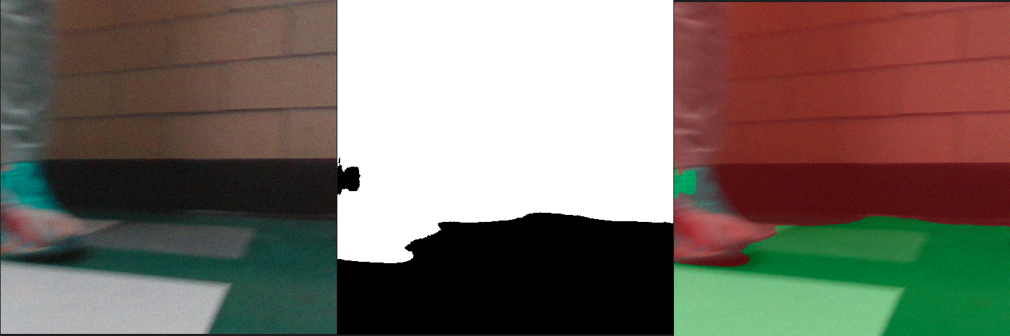
In the image below, the robot is easily able to detect the wall in front of it, and is mostly able to detect the shoe. It does label a small part of the shoe as “safe” however, enough of the shoe is labelled correctly for the robot to safely navigate around it. This image had 94% accuracy using the same method as above.