3D Printed Autonomous Car Robot Build
Overview
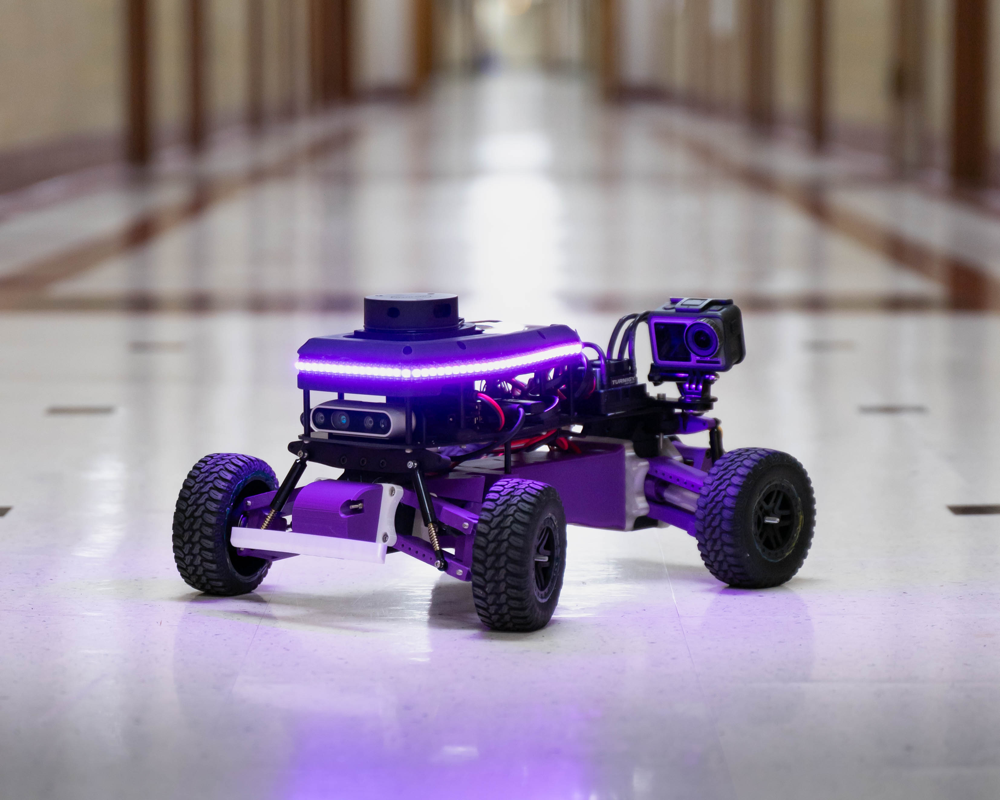
For this project, I built an autonomous car robot from scratch and programmed it to drive autonomously. I created a set of ROS 2 packages it to allow the car to drag race with traction control, drive from point to point, and race laps. I also used NVidia Isaac Sim to create an environment for testing and tuning new code before deploying it on the robot itself.
Video Demo
Project Objectives
This project had several goals that helped to set the direction of the project and guided the design process:
- Build an autonomous car robot that could be controlled using ROS 2
- Create ROS 2 packages to control the car to drive and race autonomously
- Create a well documented and reliable platform that can be used by myself and other students for future projects involving Ackermann-style robots
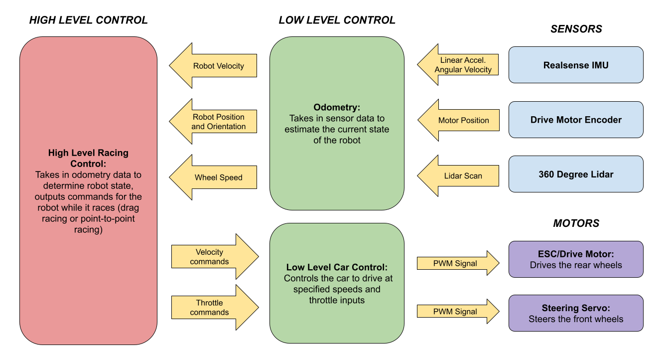
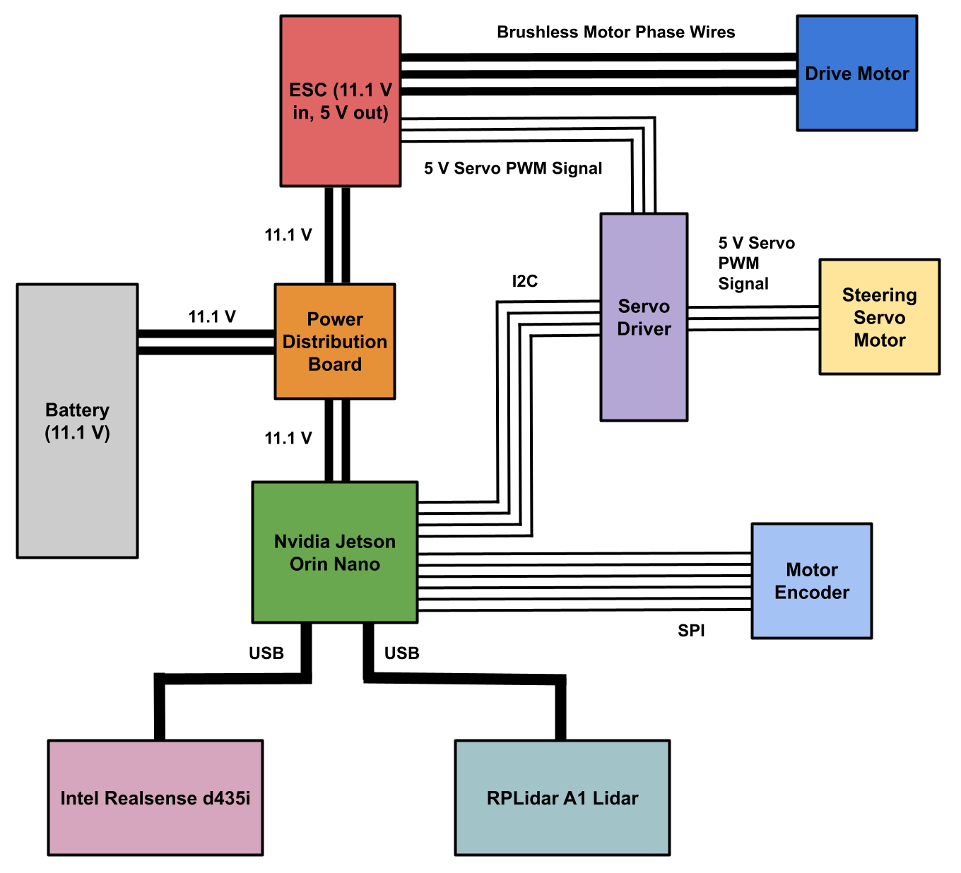
System Block Diagram
Mechanical Design
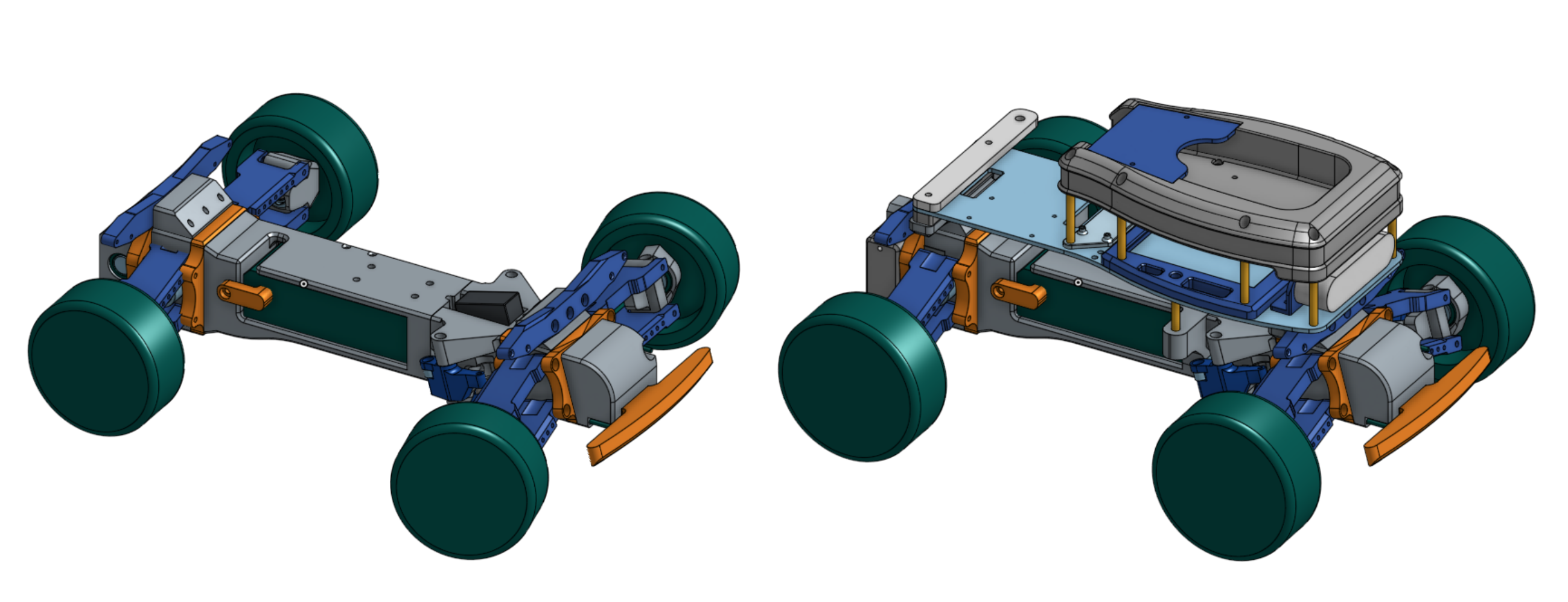
The design of this robot is based on the Tarmo5 RC car project. Tarmo5 is an open source design originally created by the YouTube channel Engineering Nonsense, which aims to design an RC car with as many 3D printed parts as possible. This design was selected due to it’s well tested nature and focus on high speed driving. In addition, the fact that the car is largely 3D printed meant that it was easy to modify and test different component designs on the car. On top of that, during testing, several parts broke due to crashes, spins, and other mishaps. Using 3D printed parts made making replacement parts quick and easy.
Below is the original Tarmo5 design in CAD on the left, along with my modified design on the right. Modifications were primarily made to accommodate mounting sensors and other electronics. The final CAD design of the vehicle can be found here.
Below are closeups of the final robot assembly. Sensors, motors, and other components are labelled with descriptions below.
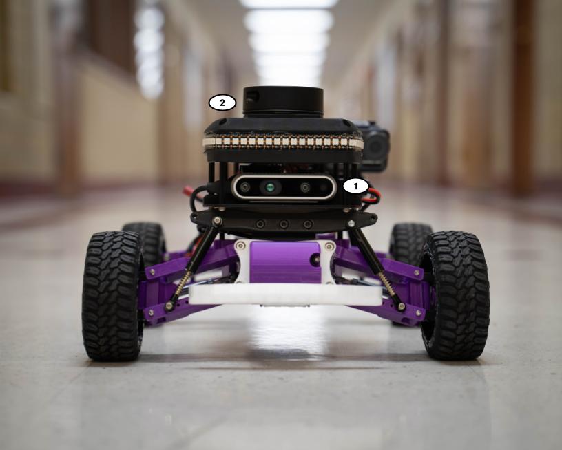
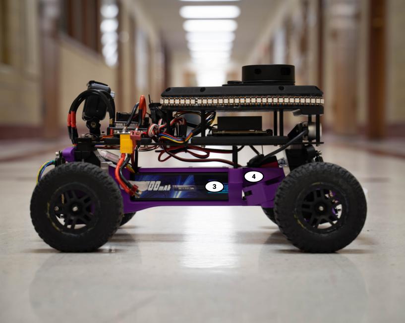
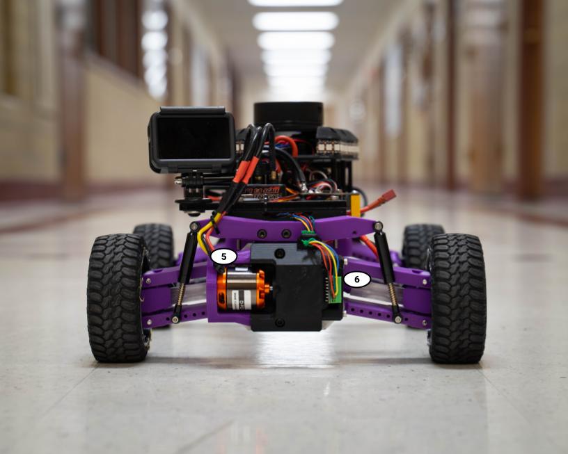
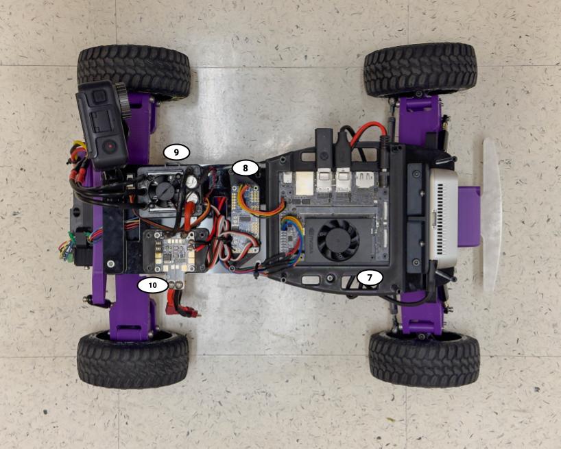
Labelled Components:
- Intel Realsense d435i Camera and IMU
- RPLidar A1 360 Degree 2D Lidar
- Battery: 5200 mAh, 11.1 V (3S LiPo)
- Steering Servo (20 kg-cm)
- Brushless Motor (650 W @ 11.1 V)
- AS5048a Magnetic Encoder
- Nvidia Jetson Orin Nano 8GB Developer Kit
- Adafruit PCA9685 Servo Driver
- Turnigy 160A 3-4S Brushless Motor ESC
- Power Distribution Board and Battery Connector
Electronics Design
This robot is controlled by an Nvidia Jetson Orin Nano 8 GB Developer Kit, a single board computer with an Nvidia GPU. The Jetson is running Jetpack 5.1.2, a modified version of Ubuntu 20.04, and Isaac ROS Humble, a GPU accelerated version of ROS 2.
Below is a simplified circuit diagram showing the electronics on the car.
Low Level Car Control and Tele-Op
The first step in getting the car to drive autonomously was controlling the throttle signal sent to the motor and the steering signal sent to the steering servo. Both the servo and the drive motor ESC use the same 50 Hz PWM signal to communicate. This control signal is used to control many RC and drone servos and motor controller. At 50 Hz, each cycle of the PWM signal lasts 20 ms. To control the servo and motor ESC, a high pulse is sent for 1-2ms fo each 20ms cycle. A signal with a pulse of 1ms/1000us commands the servo to turn fully to the right and the ESC to drive the motor at full speed in reverse, while a 2ms/2000us pulse commands the servo to turn right and the ESC to drive forward at full speed. A 1.5ms/1500us command centers the servo and stops the motor.
Because of the precise timing required for these PWM signals, a separate PCA 9685 servo driver was used to control the ESC and steering servo. It was controlled by the Jetson via an I2C connection. A ROS 2 node called control_servos was created for sending commands to the servo driver. The node subscribes to topics which carry steering and throttle commands for the motors and sends the commands to the servo driver over I2C. The servo driver then handles sending a precise PWM signal to the motor and servo.
Though the goal of this project was to drive autonomously, it was also important to be able to control the car manually. To accomplish this, another node called controller_interface was created to be able to control the car remotely. In addition, the controller interface node also allowed me to trigger services and other behaviors on the robot without being connected to a network. Because this robot can MOVE, it was easy to get disconnected from the wifi network I was using for testing. A direct connection to the robot with the controller meant that I still had the ability to stop and control the robot robot when the wifi was unreliable.
Odometry and Sensors
The robot relies on three sensors to provide feedback on it’s current state; the motor encoder, the RealSense IMU, and the Lidar.
- AS5048a Motor Encoder: A magnetic 14 bit encoder that provides feedback on the position of the motor. By taking the derivative of this value, I found the motor speed, and using the gear ratio and wheel radius, I am able to convert this to an estimate of vehicle linear velocity.
- RealSense d435i IMU: The IMU provides angular velocities and linear acceleration for the vehicle through the RealSense ROS 2 node. The gyroscope provides angular velocity feedback; this data is integrated to provide an estimate of the robot’s orientation at any given time. The linear acceleration data provided by the accelerometer is also integrated to provide another estimate of the vehicles forward speed. Both the IMU and encoder speed estimates are used to estimate the vehicles true speed, position, and orientation.
- RPLidar A1 360 Degree 2D Lidar: The scanning lidar is used to provide feedback about how far away obstacles around the vehicle are. This is used for creating maps with SLAM (simultaneous localization and mapping) and is also used for lane centering when drag racing.
To address issues with wheel slip and IMU drift, I blended the IMU speed estimate and the wheel encoder speed estimate using a complementary filter. By blending the two estimates, I avoided the downfalls of both; the IMU data stopped the short term inaccuracy in the encoder estimate when the wheels spun, while the encoder estimate prevented IMU drift in the long term. This blended odometry estimate was calculated and published by the odometry node. Below is pseudocode for the complementary filter.
Complementary Filter:
v_imu: the velocity estimate from the IMU
v_encoder: the velocity estimate from the encoder
a: the blending coefficient
v_odom: the output odometry velocity

v_odom = (a * v_imu) + ((1 - a) * v_encoder)
Velocity Control
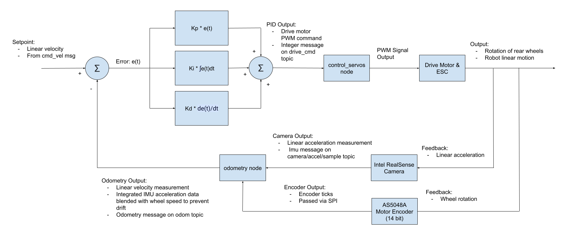
To control the robot to drive at a specific linear speed, I created a velocity_control node, which uses a PID loop to control the car’s speed. The details of this loop can be seen in the diagram below. In summary, the node takes in a reference velocity command and uses the blended odometry feedback from the odometry node and a PID loop to command the robot to drive at the specified speed.
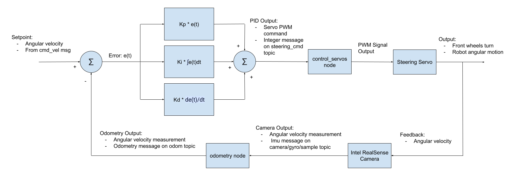
Additionally, the velocity control node can command the vehicle to drive at a specified angular velocity. This was used extensively throughout all autonomous driving tasks. This does not use any sensor blending, just the angular velocity estimate straight from the IMU. Below is a diagram of the angular velocity control loop.
Simulation in Nvidia Isaac Sim
I created a simulation of the robot in Nvidia Isaac Sim for testing and tuning new code before deploying it on the robot. This proved to be a very challenging task, largely due to tire dynamics. Tires are notoriously difficult to model, with temperature variations, slip angles, load, and more all playing a role in the amount of grip they can provide. I was able to model a tire in the simulation, but exactly matching the true dynamics of the real tire is essentially impossible without extensive testing of the tires on the robot. That being said, the simulation was more than accurate enough for testing and tuning code functionality.
First, a URDF description file for the robot was created. The URDF includes links for the wheels, sensors, and body of the car using meshes exported from OnShape. It includes joints for not only the wheels and steering, but also for the suspension. Below is the model from the URDF being manipulated in RViz.
Next, environment in IsaacSim was created and the URDF was imported. Joint limits, stiffnesses, and damping were defined, along with other physics properties such as the tire dynamics. Additionally, simulated sensors were created to replicate the real sensors discussed in the odometry section. Isaac Sim has an easy to use ROS 2 Bridge which made integrating with my packages relatively straightforward. Below you can see the robot driving in the simulation with tele-op control.
Drag Racing
The first autonomous driving challenge I decided to tackle was drag racing through hallways of the Northwestern Tech building. While this may seem like a simple task at first, trying to drive as quickly as possible makes this much more difficult. There were two main challenges: making sure the car does not run into the hallway walls and trying to accelerate as quickly as possible while not spinning out the rear wheels and loosing control.
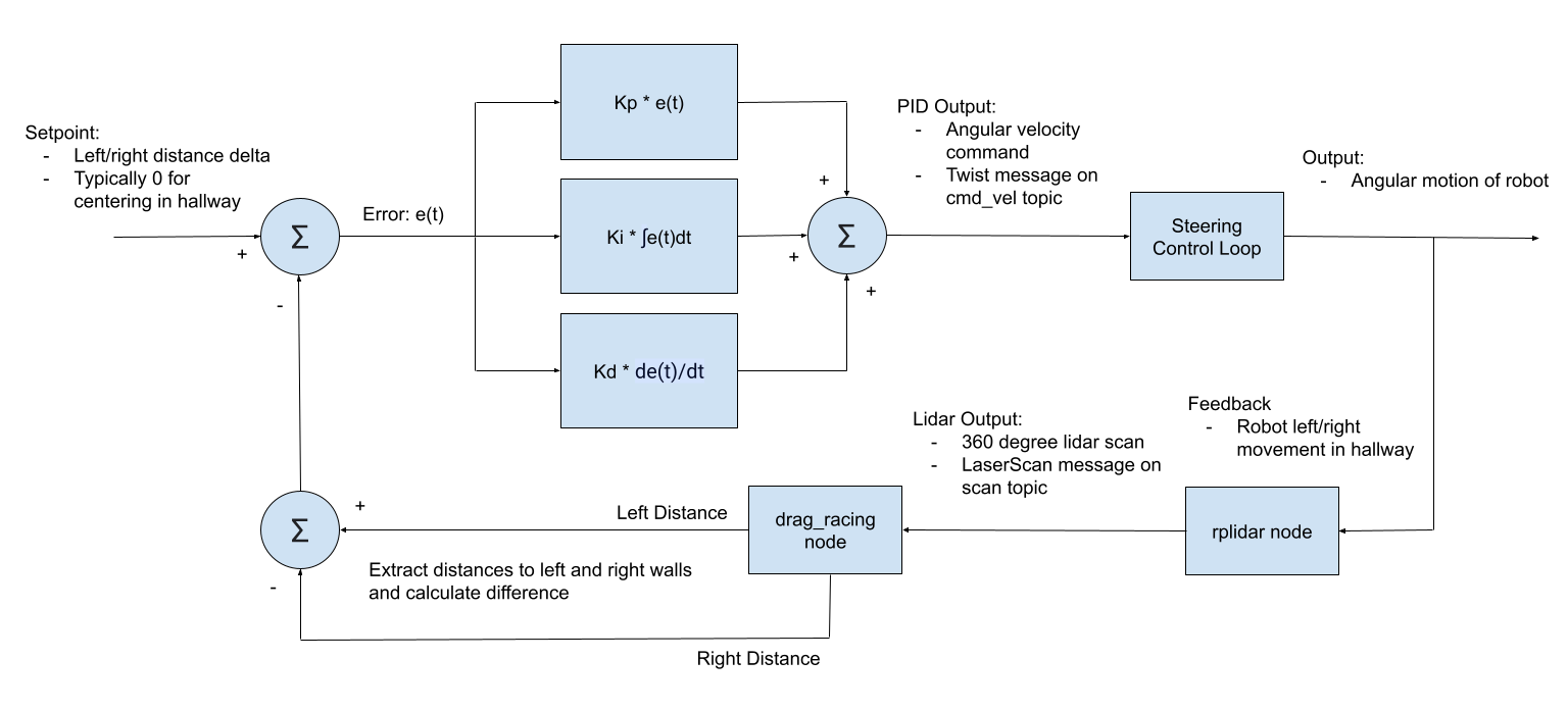
To tackle the problem of crashing into walls, I used the lidar sensor mounted on the robot. Rather than using SLAM or some other more complex localization technique, I took a sample measurements directly from the lidar scan and used them to calculate angular velocity commands for the robot. By taking a sample of points from the left side, a sample of points on the right side, finding the average of each, and then computing the difference, I was able to estimate the robot’s relative position relative to the center of the hallway. I used that difference value as input for a PID control loop which ultimately controlled the robot’s steering. A diagram of the PID loop can be seen below.
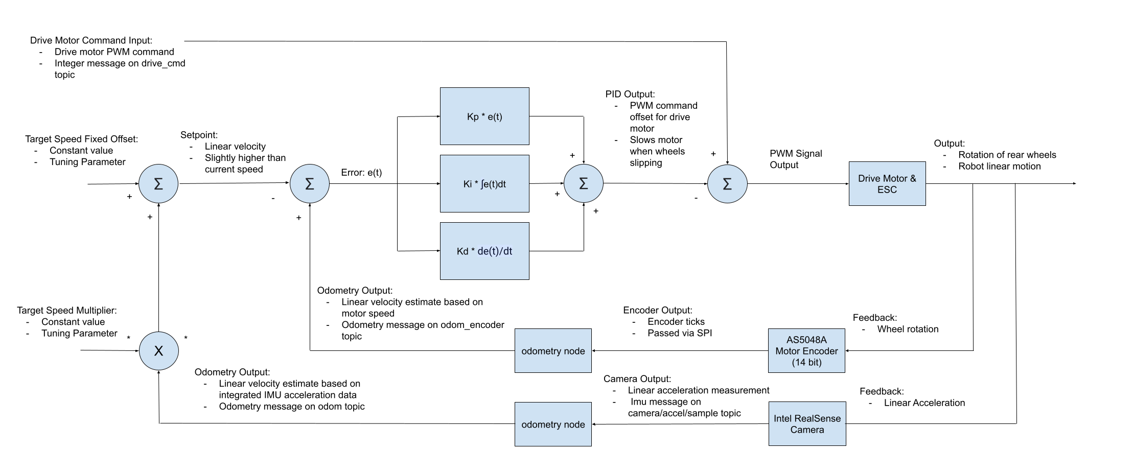
To address the wheel spin issue, I added a traction control loop to the control_servos node. I initially tried to simply ramp the throttle inputs to the robot to avoid spinning the wheels too quickly, however I found that it was difficult to find an ideal throttle curve. The throttle inputs required vary every launch, as every launch is slightly different. My traction control system compares the integrated integrated IMU velocity and the velocity estimate from the encoder on the motor to determine if the wheels are slipping. It then corrects the command being sent to the motor to a lower speed to reduce the wheel spin. A diagram of the full control loop is shown below.
Unlike other velocity control modes in this project, the traction control mode does not use blended IMU and encoder data for odometry. This is because it generates a response based on the difference between those two values, so blending them was found to lead to a worse response. Because drag racing is so short, there is not enough time for the IMU drift to come into affect, so the blending is not really needed in the first place.
Tuning these systems to work well together and drive the car quickly to the end of the hallway was a difficult task. Both systems detailed here, along with the lower level control systems, needed to work in harmony for the car to make it to the end of the hallway. Here is a sample of the less successful runs from the tuning process:
Point to Point Driving
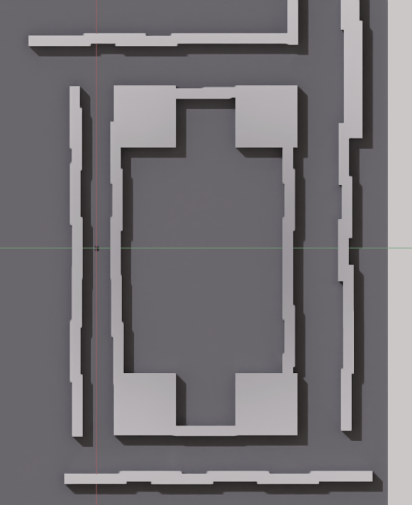
Finally, a point-to-point driving mode was implemented for driving a “race track”. This mode uses the ROS 2 Slam Toolbox package to first create a map of the environment where the car will be racing. Slam Toolbox reads the lidar scan data and the odometry data published by the odometry node and uses it to create a map of the robot’s environment. This requires driving the car slowly through the environment, often more than once, in order to create a detailed map. When creating loops through hallways for driving laps, I found it especially important for the algorithm to achieve loop closure, allowing it to realign features of the map to ensure everything lines up correctly. See an example of this below from a map created in the Isaac Sim environment. An overhead view of the simulation environment is shown below for comparison.
Once an accurate map is generated, it can be saved using the start but”ton on the controller. The next step in this process is planning the actual race path. This again involves slowly driving the car along the path you want it to follow. Once you reach the end, the desired path can be saved as a CSV file containing all the poses of the robot in the path. Now the robot is ready to drive the path.
When the path racing launch file is run and the race is started, the robot first checks it’s current position in the map based on the estimate from Slam toolbox. It determines which pose in the planned path it is currently closest to based on the Euclidean distance. Then, it takes the pose two poses ahead in the path and sets that as the target pose. It determines the difference between the robot’s current orientation and the upcoming target orientation, then uses a PID control loop to generate an angular velocity command based on that difference. This is then sent to the velocity control node, and the process repeats.
Throttle control works in a very similar way. The robot first looks at a pose 6 poses ahead of it’s current closest pose in the path. It calculates the difference in heading, then use a Proportional controller to set the throttle signal. The goal is to slow the robot down well before it reaches a corner to avoid loosing control. When going straight, it slowly ramps the throttle speed, limiting wheel spin and ensuring the robot makes it to the end of the path. This is a fairly simply method of path following that may not work well with a more complex path. However, it works well enough for navigating hallway environments with simple 90 degree corners. See the example below.
This navigation was also tested on the real robot, and the results can be seen in the video demo. Both slam and path planning are much noisier outside the sim and will require additional tuning to optimize performance.
Path Optimization
To create the most efficient for the robot, I created a path optimization function that worked by minimizing turn radii and maximizing straight segments. This function iteratively adjusts the positions of the poses in the path recorded by the robot when planning a racing path. The optimization process considers the angular difference between the segments created by consecutive poses and attempts to smooth these by slightly shifting the waypoints. The algorithm also ensures the path remains within navigable space by checking for obstacles within a certain radius of each pose. The robot uses the costmap generated during the SLAM mapping phase to determine if a given location is safe or unsafe.
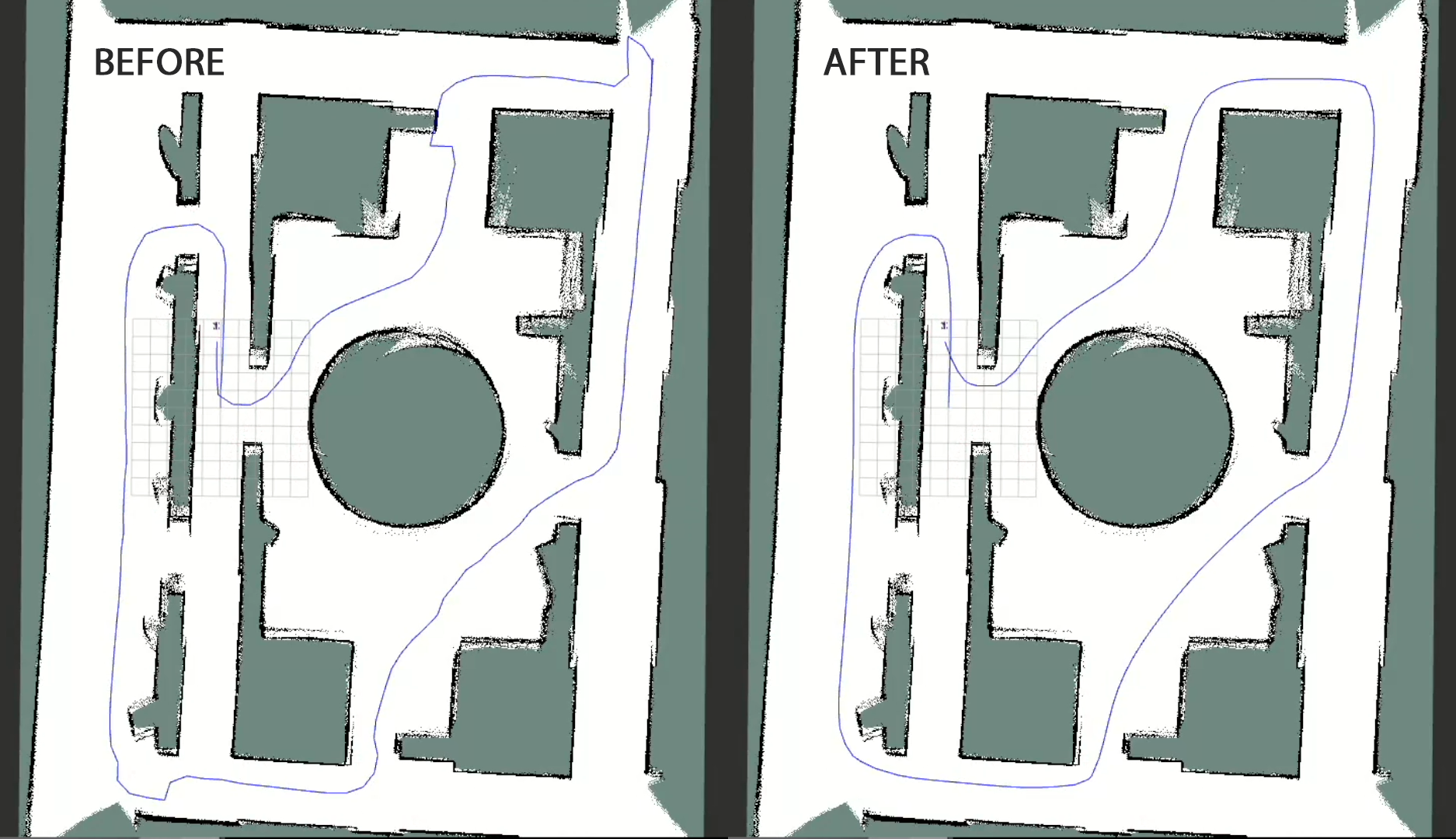
This optimization aims to produce a path that is easier for the robot to follow, with fewer sharp turns and more consistent straight lines. It also removes errors in the path that are the result of the robot relocating itself during the planning process. These changes allow the robot to travel as fast as possible when racing from point to point. Below is an example of the robot planning a path through a complex environment. Additionally, there is a comparison of the raw path and the optimized path saved by the robot.
Conclusions and Future Work
Overall, this project was very successful. I built the robot from scratch and created packages to drag race at high speed, map environments with SLAM Toolbox, and plan and drive paths with the robot. That being said, there is still lot’s that can be done with this platform. Some things I would still like to improve are:
- Faster autonomous driving
- More accurate physics simulation in Isaac Sim
- Significant tuning and development of the path following algorithm
- Use reinforcement learning to further optimize car behavior at high speeds
I have also been working on a visual odometry solution for this robot use a neural network. This allows the robot to detect walls and other obstacles using the RealSense camera, then navigate away from them. Read more about this project here.