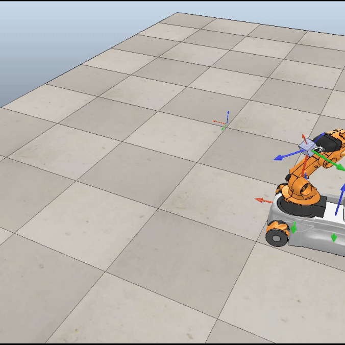
Youbot Mobile Manipulation Simulation
Overview
This project aims to control a Youbot to pick and place a block with user-specific positions and then simulate it in Coppeliasim. The algorithm first generates a reference traject of the end-effector and then applies feedback control to manipulate the Youbot.
Video Demo
Results
Two different controllers were simulated and their performance was compared. Video of the simulations with both controllers can be seen at the top of this page.
- Best: a result with a well-tuned controller with using feed-forward and PI control:
- A feed-forward-plus-PI controller with a Kp of 25 and a Ki of 0.1 was used. The error plot is shown below:
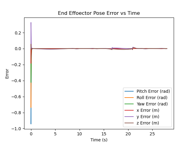
- A feed-forward-plus-PI controller with a Kp of 25 and a Ki of 0.1 was used. The error plot is shown below:
- Overshoot: a result with a poorly-tuned controller using PI control only (no feed-forward):
- A PI controller with a Kp of 5 and a Ki of 1 was used. The error plot is shown below:
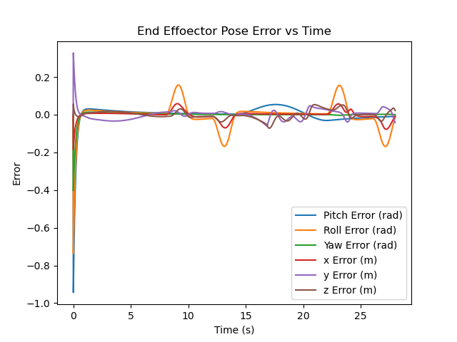
- A PI controller with a Kp of 5 and a Ki of 1 was used. The error plot is shown below:
Simulation
The NextState function calculates the robot’s configuration at the next time step based on the current configuration and the commanded joint speeds. The new configuration is calculated using the first-order Euler method. A time step of 0.01 seconds was used.
The TrajectoryGenerator function outputs a trajectory for the end-effector to pick up and place the box. The generated trajectory is provided as a list of transformation matrices for the end-effector with respect to the space frame. The function requires the following transformation matrices as inputs:
- Tse_init: The initial position of the EE relative to the space frame
- Tsc_init: The initial position of the cube relative to the space frame
- Tsc_final: The desired final position of the cube relative to the space frame
In the output trajectory, the end-effector move through the following 8 stages of the simulation:
- The EE moves from its initial configuration to a “standoff” configuration a few cm above the block.
- The EE moves down to the grasp position.
- The EE closes on the box.
- The EE moves back up to the “standoff” configuration.
- The EE moves to a “standoff” configuration above the final configuration.
- The EE moves to the final configuration of the object.
- The EE releases the box.
- The EE moves back to the “standoff” configuration.
For stages where the robot platform or arm move (as opposed to just the gripper), the algorithm uses the ScrewTrajectory function from the Modern Robotics Python library. The function takes in transformation matrices for the start and end positions of the gripper. It generates a discrete trajectory as a list of end-effector transformation matrices using the third-order/ fifth-order polynomial time-scaling method.
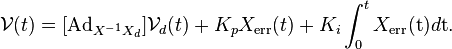
The FeedbackControl function is used to command the robot to follow the generated trajectory. Joint commands for the arm joint and the wheels are calculated using the kinematic task-space feed-forward plus feedback control law, shown below. Using this method allows for the robot to correct for error in it’s current position while also anticipating the upcoming movements in the trajectory.
Initial Configuration
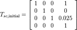
- The initial cube position in space frame is:
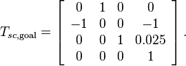
- The final cube position in space frame is:
- The initial configuration of the robot is:
```shell [-1, -0.5, 0.2, 0, -0.2, -0.6, -1.578, 0, 0, 0, 0, 0, 0] ‘’’
Joint Limit Detection
Joint limits are monitored by the CheckJointLimits function. This function checks if the next joint positions are outside the allowable range for the robot. If they are, it sets all values on the corresponding line of the Jacobian equal to 0. This ensures that the joint that is at it’s limits is not updated with a new position and does not pass the limit. The new Jacobian is returned and used to find the next set of velocity commands for the robot. The robot is more likely to enter strange poses and collide with itself when joint limits are turned off. Though the robot is also sometimes able to stay closer to the target Tse_d when it is allowed to ignore joint constraints, this is obviously not practical in the real world.