Implementation and Assessment of a Particle Filter for Robot Localization

Overview

The goal of this project was to use a particle filter to improve localization accuracy for a robot in a test environment. Odometry data containing the commanded linear and angular velocities, distance and heading measurements relative to known landmarks, and ground truth position data for the robot were all provided as part of the data set. The data was collected from robots at the Autonomous Space Robotics Lab at the University of Toronto. Thorough documentation of the robot platform, task and file formats, as well as video, are provided here: http://asrl.utias.utoronto.ca/datasets/mrclam/index.html.

Overall, the particle filter was successfully able to combine the odometry data and the measured position data to dramatically improve the position estimate relative to the pure dead reckoning estimate. As expected, the filtering algorithm still struggled in situations where no measurements were taken. However as long as measurements were taken regularly, the filter was able to keep the position estimate within ~0.25m of the ground truth position.

Results and Assessment of Filter Performance

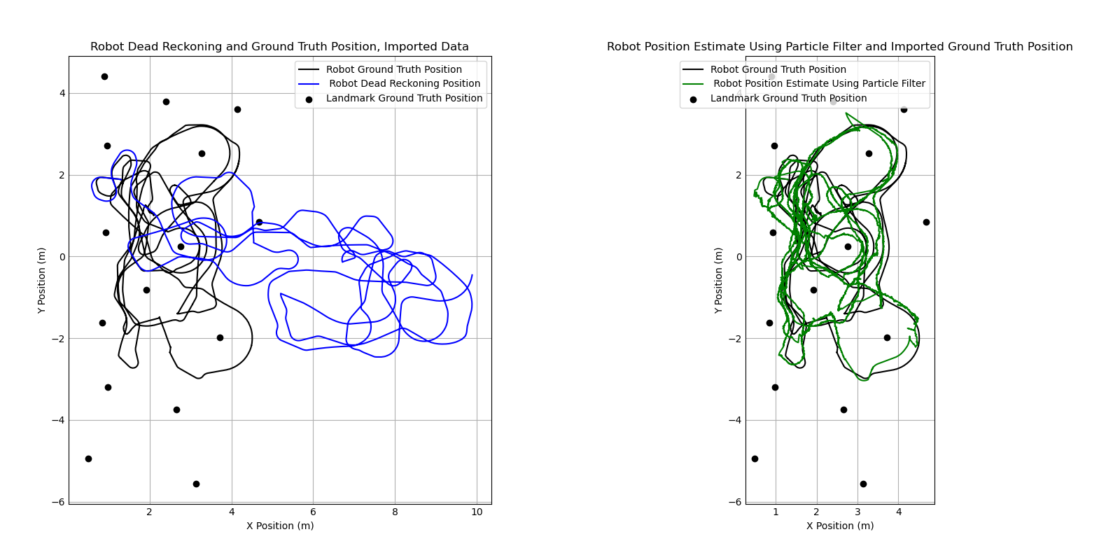
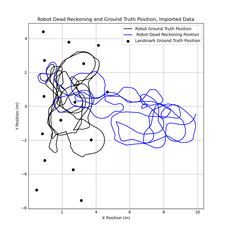
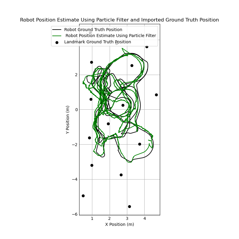
When comparing the particle filter output to the output from the pure dead reckoning model, there is a significant difference between the position estimate using the particle filter and the estimate using dead reckoning. Whereas the dead reckoning estimate drifted far away from the correct position and was effectively outputting a random θ, the particle filter estimate generally stayed very close to the ground truth position for the entire run of the robot. However, compared to the dead reckoning estimate, the position data is noticeably noisier. This makes sense intuitively, as the particle filter estimate is a representation of a probability distribution which will shift as new information is fed through measurements. The position estimate jumps around as it responds to new measurement data, while the dead reckoning is purely a function of the input and previous position; there is no uncertainty, and therefore no noise.

This is further corroborated by the error plot below. The estimates from the particle filter have more noise, but they stay much closer to the ground truth values. The position error for the particle filter estimates is consistently below 0.25 meters, while the dead reckoning data smoothly drifts to 7+ meters of error.

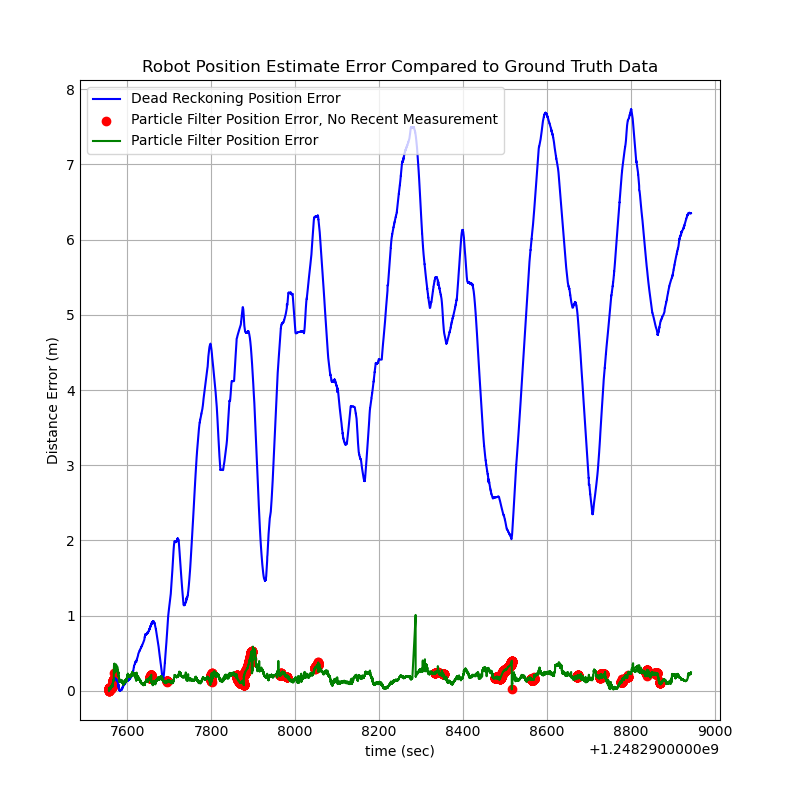
At several points, the error on the particle filter spikes noticeably. Many of those points are marked in red, indicating that at that time, the robot had not received a measurement for more than one minute. It makes sense that error would increase at those points, as the robot is not taking in any measurement data to correct for its dead reckoning drift. To improve performance, it would be ideal for the robot to constantly be taking in useful positional information that it can use to correct its position estimate.

Dead Reckoning Motion Model

The dead reckoning position estimate based on simple trigonometry and physics. The inputs for the model are the linear velocity and angular velocity (omega) commands provided in the odometry data file, along with a time interval between commands.

First, the program determines whether the current command is for a linear movement or not based on the angular velocity. If angular velocity equals zero, the movement is assumed to be linear. For linear motion, the angle of the robot relative to the environment (theta) does not change. The distance the robot travels is simply calculated using the velocity and time interval.

distance = vel * time

For a non-linear movement, where angular and linear velocity are not zero, the robot is assumed to be moving in a curved path. Linear and angular velocity are considered to be constant for each robot movement, and moving with a constant linear and angular velocity will result in movement in a circular path. To determine the position of the robot after executing the command, a radius of curvature is calculated using the equation below.

radius = abs(vel / omega)

The change in the robot’s angle relative to the environment is calculated by multiplying the the angular velocity by the time interval. This is then added to the current theta angle to find the new theta angle.

Δtheta = omega * time

theta_new = theta_current + Δtheta

Next, the center of the curve is calculated using the equations below. The curve center is assumed to be one radius to the left or right of the robot, depending whether the robot is turning to the right or left.

Left Hand Turn:
curveCenterX = x_current + radius * cos(theta + pi/2)
curveCenterY = y_current + radius * sin(theta + pi/2)

Right Hand Turn:
curveCenterX = x_current + radius * cos(theta - pi/2)
curveCenterY = y_current + radius * sin(theta - pi/2)

Finally, new x and y coordinates are calculated using the equations below. Essentially, these equations determine the robot’s position along the curve with the center and radius calculated above based on the calculated Δtheta.

Left Hand Turn:
x_new = curveCenterX + radius * cos(theta_new)
y_new = curveCenterY + radius * sin(theta_new)

Right Hand Turn:
x_new = curveCenterX - radius * cos(theta_new)
y_new = curveCenterY - radius * sin(theta_new)

Measurement Model

The measurement model uses trigonometry to estimate the distance and heading from a specified state of the robot to a known landmark position. Within the particle filter, it is used to estimate the distance and heading from any given particle to a landmark and a specified x-y position.

The inputs for the model are the current state of the robot or particle (x, y, and theta) and the position of the landmark (x and y). To calculate the distance between the robot state and the landmark, Pythagorean’s theorem is used. To calculate the heading angle from the robot to the landmark, phi, in the global coordinate system, the arctangent of the y distance between the robot and the landmark over the x distance between the two is used. The robot orientation theta is then subtracted to convert the heading from the global coordinate system to the robot’s coordinate system, as that is what the robot would report if it took this measurement. The full equations for both calculations are below.

dist = sqrt((x_robot - x_landmark)**2 + (y_robot - y_landmark)**2)

phi_global = atan((y_robot - y_landmark)/(x_robot - x_landmark))

phi_robot = phi_global - theta

The outputs are the distance from the robot to the landmark and the heading of the landmark relative to the robot frame, phi_robot. This is the same data that is reported by the sensor system on the robot, so the outputs from this model can be compared to a current measurement from the sensor to evaluate the current position of the robot.

Implementation of Particle Filter

Below is an explanation of the basic operation of a particle filter.

First, an initial belief state is generated. In the particle filter, the belief state is comprised of a set of particles, X_t. Each particle represents a possible state of the robot. In this project, the state variables are the robot coordinates x and y and the orientation theta. The initial particle set can be generated using a uniform distribution across the entire workspace, a random distribution, or they can be generated based on the initial robot state, if it is known. The initial state is be called X_t−1. The number of particles (M) is specified as part of the filter design.
Next, the robot will take a measurement to estimate its state. The measurement, z_t, is used to calculate the importance factor for each particle in X_t−1. The filter will then estimate the expected measurement for each particle using the measurement model. Then, it will compare the expected measurement for each particle to the measurement z_t. Particles whose estimates more closely match the measurement are assigned high probabilities, while particles that do not match are assigned low probabilities. These probabilities are called importance factors, ω_t. The state of each particle, along with the importance factor, is then added to a new matrix X′_t.
Then, the particle set is re-sampled based on the importance factors. From the particle set X′_t, particles are sampled randomly with the importance factors as weights (i.e. particles with high importance factors are more likely to be selected). The selected particles should be added to the new belief state X_t. There will be redundant particles, as particles with high importance factors will be sampled more than once. This new particle set should have a distribution with more particles in the most probable states as a result of this resampling step. This resampling is critical for estimating the robot’s state successfully.
Finally, wait for a new measurement to repeat the process. X_t is now the current belief state is now. While waiting for a new measurement, X_t may still be updated based on inputs to the robot. In this project, the state of every particle in the belief state is updated between measurements based on the odometry input data provided between the measurements and using the motion model. When a new measurement z_t is collected, X_t becomes X_t−1 and the process repeats.

For this implementation, a few changes were made to the basic particle filter described above. In this filter, the filter generates a set of random initial particles when the first measurement is taken. The initial number of particles is specified in the tuning parameters; 200 initial particles was found to work well. These particles are all generated around the initial position of the robot. The x and y positions of the particles are generated using these equations.

x_particle = (rand(-1,1) * initialSpread) + x_robot
y_particle = (rand(-1,1) * initialSpread) + y_robot

Where rand(-1,1) represents a random number between –1 and 1. The variable initialSpread is the maximum x or y distance that the generated particle can be from the current position estimate. It is a tuning parameter specified by the user. An initial spread of 0.25 m was found to be optimal in this project. The theta angle of the particles is generated using the equation below.

theta_particle = (rand(-1,1) * initialTurn) + theta_robot

The variable initialTurn is the maximum change in the theta angle between the generated particle and the current position estimate. An initialTurn of π/8 radians was found to work well in this project. These variables are then added to the current belief state array. This is repeated until the full set of particles are generated.

When a measurement to a specified landmark is received, each particle is run through the measurement model described above, which outputs a distance and heading (phi) from each particle to the landmark measured. The position of the landmark in the global frame is known. To calculate the probability for each particle, the distance between the estimated position of the landmark relative to the particle and the landmark position measured by the robot are calculated using Pythagorean’s theorem. This distance is the error between the particle’s estimate of the landmark position and the true landmark positions, and is used for calculating the probability each particle is correct. Smaller error values correspond with particles that are more likely to match the true state of the robot. The equations are shown below.

x_landmark_particle = dist_particle * cos(phi_particle)
y_landmark_particle = dist_particle * sin(phi_particle)
x_landmark_measured = dist_measured * cos(phi_measured)
y_landmark_measured = dist_measured * sin(phi_measured)
landmark_position_error = sqrt((x_landmark_measured - x_landmark_particle)**2 + (y_landmark_measured - y_landmark_particle)**2)

The distance between the estimate and the measurement is then divided by a variable sigma. Sigma represents represents the uncertainty of measurements from the sensor, but it is treated as a tuning parameter within the context of this project. The distance estimate and sigma are used to calculate a z-score, which represents the number of standard deviations that the estimate is from the measurement. This can then be converted to an approximate probability using the following equations.

zScore = landmark_position_error / sigma
probability = 2 * (0.5 * exp(-zScore**2 / 2))

Once all the particles have probabilities calculated, the highest probability particles are selected. The number of particles to select is a tuning parameter; 30 was found to work well in this project. The average x and y positions and θ angle are calculated for the high probability particles. The probability for the average particle is also calculated based on the average probability of all the high probability particles. This average particle is then considered to be the new overall position estimate.

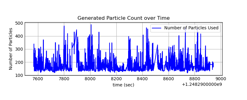
Next, the new particle set is generated. The number of particles is based on the probability of the high probability average particle. This means that when the model is more confident, fewer particles are created to improve compute time. When the model is less certain, more particles are generated to improve accuracy. The number of particles is calculated using the equation below.

num_particles = (1 - prob_avg) * (particles_max - particles_min) + particles_min

The minimum and maximum particles are tuning parameters; 100 and 500, respectively, have been found to work well. The variable particle count is implemented to improve compute times for the model. Once the model is confident in its position estimate, it can use fewer particles to speed compute time while still maintaining an accurate model. If uncertainty increases due to fewer measurements or drift, more particles are generated. Below is a graph of the number of particles generated during the full run of the filter.

Next the new particles are generated. Rather than selecting particles from the belief state and copying them to the new belief state, this model selects a particle randomly with weighting from the calculated probabilities. It then generates a new particle near the selected particle and adds the newly generated particle to the new belief state. The new particles are generated using the equations below.

x_new_particle = (rand(-1,1) * newSpread) + x_random_particle
y_new_particle = (rand(-1,1) * newSpread) + y_random_particle
theta_new_particle = (rand(-1,1) * newTurn) + theta_random_particle
newSpread = maxNewSpread * (1 - prob_random_particle)
newTurn = maxNewTurn * (1 - prob_random_particle)

The variable newSpread is the maximum x/y distance the new particle can be from the old particle. Likewise, newTurn is the maximum change in θ between the new particle and the old particle. The values of newParticleSpread and newParticleTurn are calculated based on the inverse of the probability of the random particle that the new particle is based on. This means that if a random particle with a high probability is selected, the generated random particle will be very close to the position of the random particle. If the random particle is low probability, the generated random particle is allowed be further away. This helps address th issue of particle deprivation. Because there are always new particles being generated, the particle set will never be taken over by one or two particle estimates, which is an issue when particles are simply duplicated.

From there, the belief state is updated with the new particles. Until a new measurement is registered, the model will move both the high probability average estimate point and every particle in the belief state according to the motion model and the odometry data. When there is a new measurement, the process will be repeated by calculating probabilities for the existing particles, selecting a new high probability average point, and generating another new particle set.

GitHub