Using the A* Algorithm to Plan Paths and Avoid Obstacles
Overview
The goal of this project was optimizing a robot’s navigation around obstacles using the A* (A Star) algorithm. A* is a artificial intelligence method that helps the robot decide its best path. Throughout the project, I explored an adaptive “online” version of the algorithm, which deals with obstacles discovered while the robot is moving. This meant that the robot could not react to some objects until it was very close to them. Another challenge was implementing a PID controller to enable the robot to follow the path found by the A* algorithm. This controller
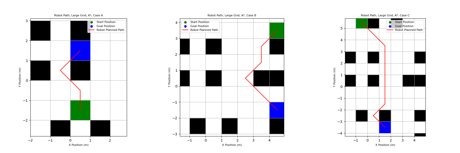
Basic A* Planning
The A* algorithm is used in this assignment to find a path between two cells on a grid while navigating around cells that contain obstacles. This algorithm uses a heuristic equation to direct its search toward the goal cell, as opposed to uniformed search algorithms which would search equally in all directions. The current and goal cells are both known, allowing the heuristic to be used to direct the search toward the goal.
The robot is able to move to any of the eight cells that surround it, and the algorithm determines which cell to move to next by estimating the total distance to the goal if it moves in each direction. It does this using the equation below:
f = h + g
The estimated total cost from the start to the goal is given by f, g is the cost of moving from the start cell to the cell being evaluated, and h is the estimated cost of moving from the cell being evaluated to goal cell. The variable g is calculated by adding the cost of moving from the current cell to the cell being evaluated and the cost of moving from the start cell to the current cell. The cost of moving to an open cell is given as 1, while moving into a cell occupied by an obstacle is 1000. The high cost of movements into cells with obstacles is what allows the algorithm to navigate around obstacles. Below are the paths output by the algorithm for three different start and goal locations on the grid.
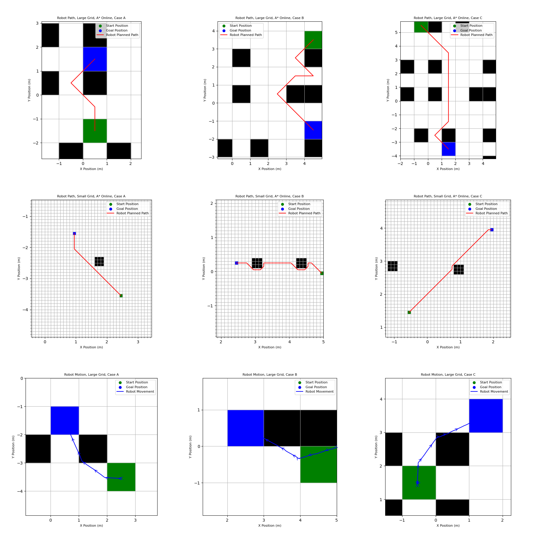
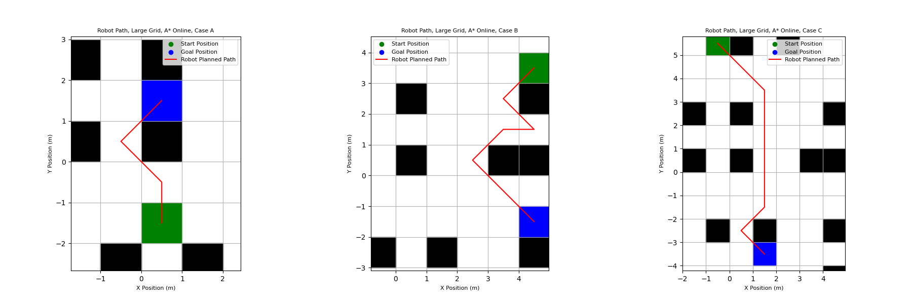
Online A* Planning
The A* “online” algorithm functions very similarly to the standard A* algorithm, with the main difference being whether the position of obstacles are known to the robot. With the standard A* algorithm, all the obstacles are known to the robot and the start of the planning process. This means it can successfully plan paths around obstacles without being directly adjacent to them. With the online algorithm, the robot does not know where obstacles are located until it is in the cell directly adjacent to the cells they occupy.
Because the obstacles are not known to the robot until it is near them, the algorithm needs to be run again after every step of the robot in case any new obstacles were detected. This means that the expanded set of nodes is essentially reset after every movement. By the time the robot reaches the goal, the expanded set will only be the cells surrounding the final cell occupied by the robot before reaching the goal.
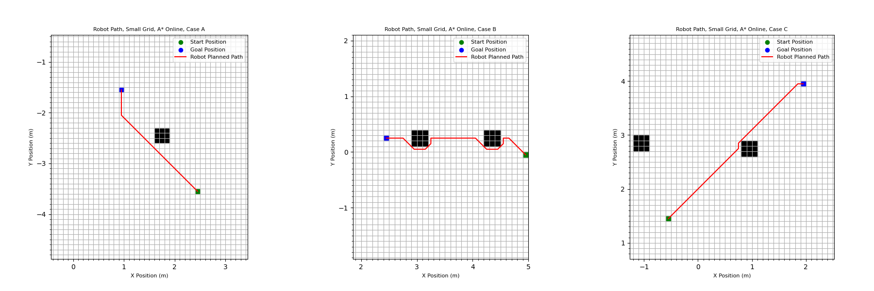
Below is the path output by the algorithm for three different start and end goal locations. They look similar to the paths output by the standard algorithm, but there are minor differences. In Case B specifically, the algorithm navigates around one obstacle, then moves down and to the right, towards the goal, before realizing there is another obstacle it needs to avoid. This demonstrates that the robot is not able to see the obstacle until it is in the directly adjacent cell when doing online planning.
Reducing the Grid Size
Next, the size of the grid squares was reduced from 1m x 1m to 10cm x 10cm. This should theoretically improve the accuracy of the algorithm, as it has more options for creating a path. Obstacles were modified to have a total size of nine squares (0.3cm x 0.3cm). Three new start and goal positions were evaluated, and the plotted paths can be seen below.
Adding Robot Motion
Next, robot motion was simulated using a kinematic controller. The kinematic controller generates odometry commands for the robot using a PID controller. The controller guides the robot from one cell to the next cell in the planned path. This function takes the robot’s current position and orientation as an input as well as the current linear and angular velocities. First, the controller calculates the difference between the robot’s current heading and the heading towards the target cell. The heading to the target cell (phi_target) is calculated using the equation below.
phi_target = atan((targetX - currentX)/(targetY - currentYS))
The difference between the current heading and target heading is the variable controlled by the PID loop. The cumulative error is also tracked, and the current error is multiplied by the time step and added to the cumulative after every cycle. This is effectively the integral of the error with respect to time.
To calculate the angular velocity command, the controller multiplies the current error, the cumulative error, and the current angular velocity by the P, I, and D control variables, which are specified by the user. The current error is the proportional variable, the cumulative error is the integral of the error, and the current angular velocity is equal to the derivative of the error. P, I, and D values of 20, 0.5, and –1, respectively, were found to work well. The velocity command is also based on the orientation error. When the magnitude of the error drops below a specified tolerance, the velocity command is set to max velocity, and the robot accelerates. If the error goes above the tolerance, the velocity command is zero.
To execute the odometry commands, the commands and the robot’s current state are passed to the execute_odometry() function. This function calculates the new position and heading of the robot after executing a command. The acceleration required to reach the commanded linear and angular velocities are calculated and taken into account. If these acceleration values exceed the user specified maximums for the robot, the acceleration is limited to said maximum. Next, based on these constrained acceleration values, new angular and linear velocities targets are calculated which do not exceed the acceleration limits.
At this point, noise could be added to the commanded angular velocity. Noise values are generated randomly based on a normal distribution between user specified values. The randomly generated noise value is added to the omega command before it is executed. The final command with the limited acceleration and added noise are the executed.
This process is repeated until the robot is within a new cell. Once in a new cell, the target is updated to be the next cell in the path and the robot begins driving toward the new target.
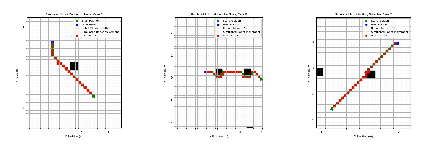
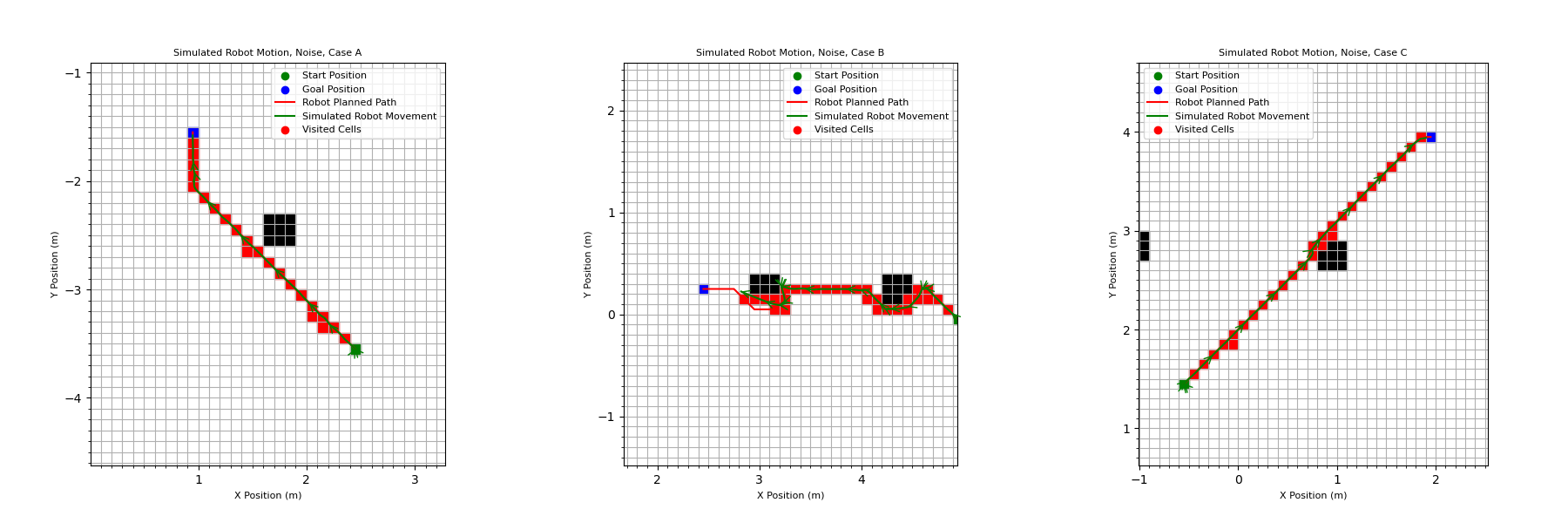
This process was repeated twice, once with noise added and once without. Both results are shown below.
Robot Motion Without Noise:
Robot Motion With Noise:
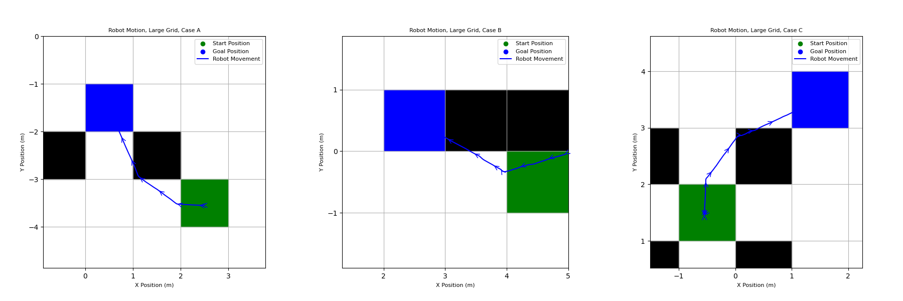
Robot Movement While Planning
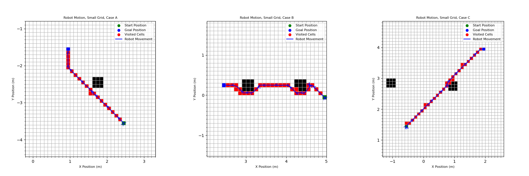
Finally, the robot was made to plan the paths while driving them. The online A* planning and the motions of the robot were both being simulated simultaneously. Because the robot motion is not perfect, it would replan it’s path any time it entered a new square, even if it was not the square that it intended to move into. This meant that the path was automatically updated when the robot made a mistake while moving. This method was run using both the fine grid and the courser grid with larger squares.
There are a couple of differences between the performance of the program when using the fine grid and the course grid. First, the movement of the robot is “smoother” when using the courser grid, with more straight-line motions. The robot also gets stuck far less. This is likely because the robot’s target and path change far less frequently than with the fine grid. Every time the path changes, the robot needs to correct its heading so it is moving in the right direction, which takes time. With the course grid, this happens less often, and therefore the full execution takes less time with fewer changes in direction.
On the other hand, the course grid is able to complete far more precise actions, moving around edges of the obstacles. In comparison and as expected, the course grid results in a simple motion that largely avoids the obstacles. It does intersect the corners of obstacle cells slightly. Both girds could be useful for different applications – the course grid would be good for making a rough path across a large, mostly open space, while the course grid would perform better for moving to precise locations and in areas with a large number of obstacles.
Robot Motion Using Fine Grid:
Robot Motion Using Course Grid: